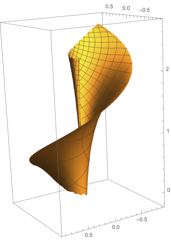
Since Joseph asked for pictures, I will add to Robert's excellent response with the following images.

For the purposes of implementing Robert's change of variables in Mathematica, I simplified the composition as shown below:

(*twist parameter*)
t = Pi/6;

(*auxiliary function*)

g[x_, y_] := Sqrt[x^2 - y^2 + (x^2 + y^2)*Cos[2*t]];

(*change of variables for u*)

u[x_, y_] := 
  Csc[t]*(Log[x^2 + y^2] - 
     Log[Sqrt[2]*x + 
       g[x, y]] + (Cos[t]*
        Log[(-(x*Sqrt[1 + Cos[2*t]]) - 
            g[x, y])/(-(x*Sqrt[1 + Cos[2*t]]) + g[x, y])])/2);

(*parameterization*)

r[x_, y_] := {Sin[t]*Cos[u[x, y]]*y/x, Sin[t]*Sin[u[x, y]]*y/x, 
   Cos[t]*(Sqrt[1 - Tan[t]^2*y^2/x^2] + 
       Log[(Tan[t]*y/x)/(1 + Sqrt[1 - Tan[t]^2*y^2/x^2])]) + 
    u[x, y]*Sin[t]};

The domain of r[x,y] is the region where $y\geq0$, $x\geq y\tan t$. This parameterization is an isometry from its domain (endowed with the Poincare half-space model metric) to its image.

First, here is an image of the parameterized surface using Mathematica's standard mesh function

r1 = 1; r2 = 10; ParametricPlot3D[r[x, y], {x, 0, r2}, {y, 0, r2}, 
 RegionFunction -> 
  Function[{a, b, c, x, y}, 
   x >= Tan[t]*y && r1^2 <= x^2 + y^2 <= r2^2], PlotPoints -> 100]

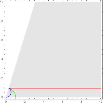
Next, let's visualize some geodesics. Below we show some geodesics in the half-plane model and their images under the parameterization.

(*parameter for paths*)
rad = 1;

(*Geodesics in half-plane model*)
path1[x_] := {x, Cos[t]*rad};
path2[th_] := {rad*Cos[th], rad*Sin[th]};
path3[th_] := rad*Sin[t]/Sin[2 t]*{Cos[th], Sin[th] + 1};

(*Show geodesics in half-plane model with domain*)
Show[
 RegionPlot[domain, {x, 0, 10}, {y, 0, 10}, ImageSize -> Medium, 
  PlotStyle -> GrayLevel[0.9], BoundaryStyle -> None],
 ParametricPlot[path1[x], {x, Tan[t]*rad, 10}, PlotStyle -> Red],
 ParametricPlot[path2[th], {th, 0, Pi/2 - t}, PlotStyle -> Green],
 ParametricPlot[path3[th], {th, -Pi/2, Pi/2 - 2 t}, 
  PlotStyle -> Blue]
 ]

Now, those same three geodesics mapped onto Dini's Surface.

Show[
 ParametricPlot3D[r[x, y], {x, 0, 10}, {y, 0, 10}, 
  RegionFunction -> Function[{a, b, c, x, y}, domain], 
  PlotPoints -> 100, Mesh -> False, PlotStyle -> Opacity[0.5], 
  PlotRange -> {{-1, 1}, {-1, 1}, {-4, 4}}],
 ParametricPlot3D[r @@ path1[x], {x, Tan[t]*rad, 10}, 
  PlotStyle -> Red],
 ParametricPlot3D[r @@ path2[th], {th, 0, Pi/2 - t}, 
  PlotStyle -> Green],
 ParametricPlot3D[r @@ path3[th], {th, -Pi/2, Pi/2 - 2 t}, 
  PlotStyle -> Blue]
 ]

The blue geodesic seems to be what Joseph was imagining in the first place, following the surface to $z=-\infty$ and getting ever closer to the $z$-axis. The green geodesic leaves the rim at a right angle and follows the shortest path to the $z$-axis. Finally, most surprising to me anyway, is the red geodesic, which winds up the surface to $z=\infty$.