added 551 characters in body
Source Link

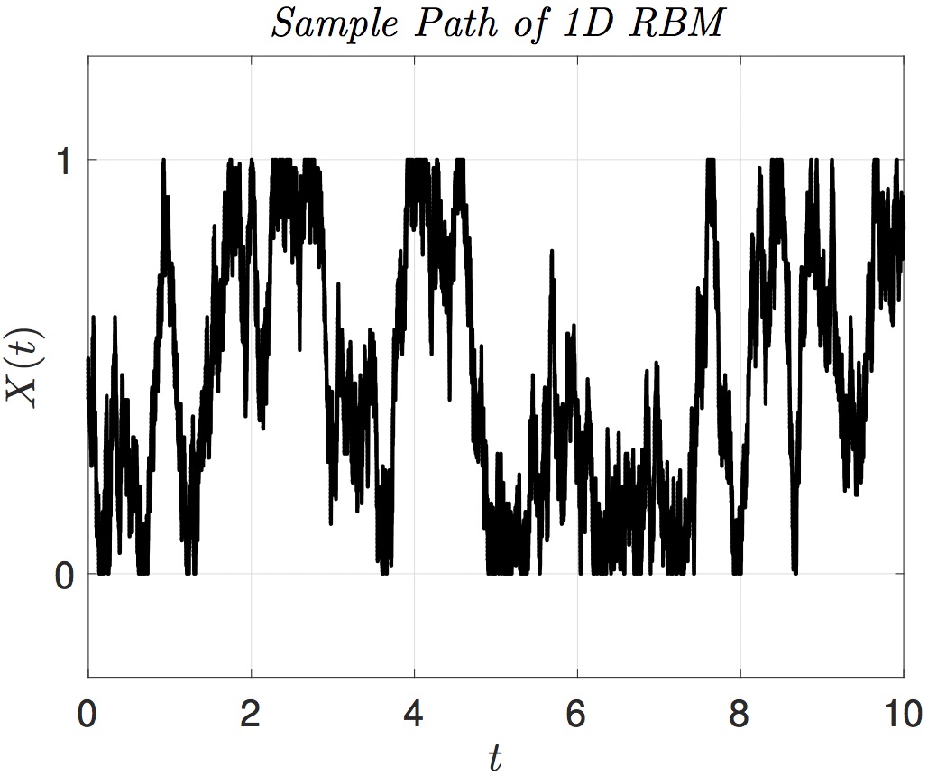
Since the components of the given planar RBM are uncoupled, it suffices to consider a scalar RBM $X$ on the spatial interval $[0,1]$. Here is a sample path of this process on the temporal interval $[0,10]$.
sample path

I will approach local time via the occupation time $$ \int_0^t 1_{[0, \epsilon]}(X(s)) ds $$ which gives the (random) amount of time the process spends in an $\epsilon$ neighborhood of zero during the interval $[0, t]$. This is a fairly complicated random variable, since it depends on the entire path of the RBM. However, its expected value is analytically available. Let $$ u^{\epsilon}(t,x) = \mathbb{E}_x \int_0^t 1_{[0, \epsilon]}(X(s)) ds \;. $$ Note that $u^{\epsilon}(t,x)$ satisfies an inhomogeneous initial boundary value problem: $$ \partial_t u^{\epsilon}(t,x) = \frac{1}{2} \partial_{xx} u^{\epsilon}(t,x) + 1_{[0, \epsilon]}(x) \quad \forall x \in [0,1] \;, \forall t \ge 0 \;, $$ with initial data $u(0,x)=0$ and pure Neumann boundary conditions $\partial_x u(t,0) = \partial_x u(t,0) = 0$. By expanding the solution and the inhomogeneity in terms of the eigenfunctions of the second derivative operator $\{ e_j(x) \}$ on $[0,1]$ with pure Neumann boundary conditions at $0$ and $1$, one obtains the following explicit solution: $$ u^{\epsilon}(t,x) = \epsilon t + 2^{3/2} \sum_{j \ge 2} \left( 1- \exp\left( \frac{t}{2} (j-1)^2 \pi^2 \right) \right) \frac{\sin( (j-1) \pi \epsilon)}{(j-1)^3 \pi^3} e_{j}(x) $$
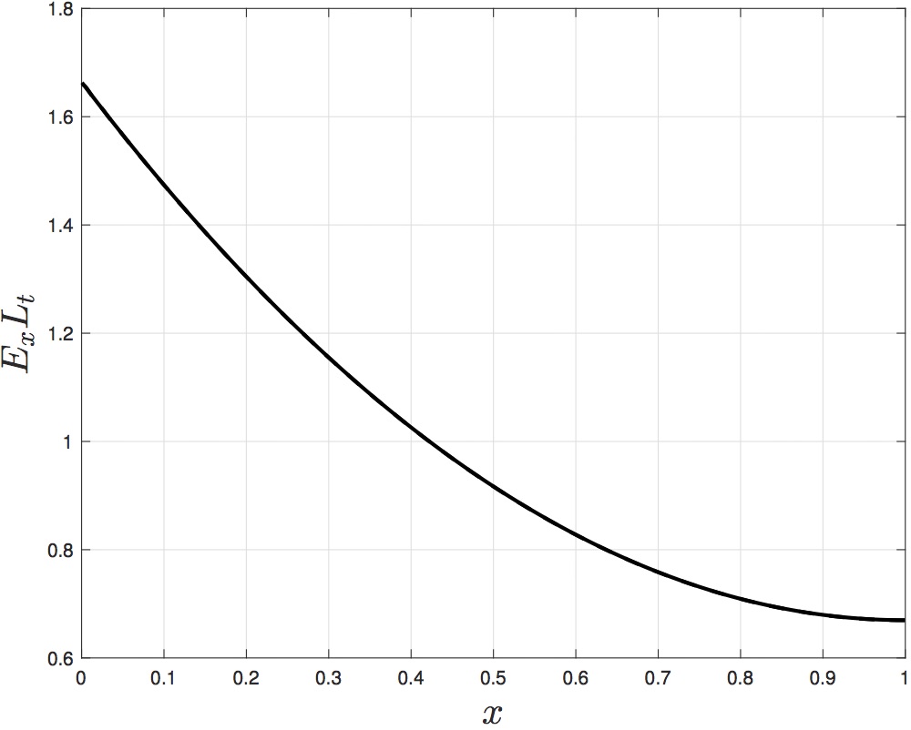
The following figure plots the behavior of $E_x L_t := \lim_{\epsilon \downarrow 0} \frac{u^{\epsilon}(t,x)}{\epsilon}$ as a function of the initial condition of the RBM $X(0)=x$ with $t=1$. As expected, this quantity decreases with distance from zero. (Since $t=1$, I find it curious that this quantity is greater than unity.)
local time

To answer the question, just view $x$ in this figure as the vertical component of the cartoon given in the question. As we already said, what happens in the horizontal component can be treated separately.

ADD

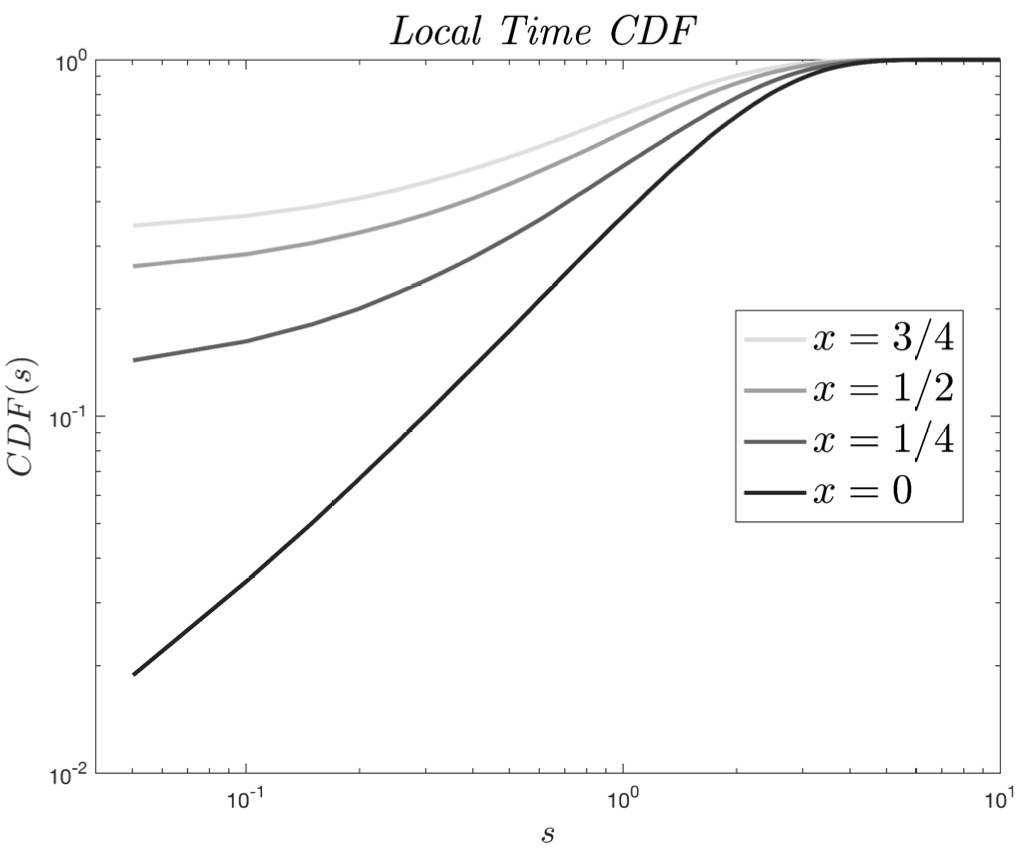
By using Monte-Carlo simulation, it is straightforward to obtain even more detail about the random variable $L_t^{\epsilon} = \epsilon^{-1} \int_0^t 1_{[0, \epsilon]}(X(s)) ds$. Here are graphs of the cumulative distribution function $CDF(s)=\mathbb{P}_x(L_t^{\epsilon} \le s)$ with $t=1$, for the initial conditions $X(0)=x$ indicated in the figure legend, and for $\epsilon$ sufficiently small. Logarithmic scaling is adopted to make it easier to compare the CDFs.
local time cdf

Since the components of the given planar RBM are uncoupled, it suffices to consider a scalar RBM $X$ on the spatial interval $[0,1]$. Here is a sample path of this process on the temporal interval $[0,10]$.

sample path

I will approach local time via the occupation time $$ \int_0^t 1_{[0, \epsilon]}(X(s)) ds $$ which gives the (random) amount of time the process spends in an $\epsilon$ neighborhood of zero during the interval $[0, t]$. This is a fairly complicated random variable, since it depends on the entire path of the RBM. However, its expected value is analytically available. Let $$ u^{\epsilon}(t,x) = \mathbb{E}_x \int_0^t 1_{[0, \epsilon]}(X(s)) ds \;. $$ Note that $u^{\epsilon}(t,x)$ satisfies an inhomogeneous initial boundary value problem: $$ \partial_t u^{\epsilon}(t,x) = \frac{1}{2} \partial_{xx} u^{\epsilon}(t,x) + 1_{[0, \epsilon]}(x) \quad \forall x \in [0,1] \;, \forall t \ge 0 \;, $$ with initial data $u(0,x)=0$ and pure Neumann boundary conditions $\partial_x u(t,0) = \partial_x u(t,0) = 0$. By expanding the solution and the inhomogeneity in terms of the eigenfunctions of the second derivative operator $\{ e_j(x) \}$ on $[0,1]$ with pure Neumann boundary conditions at $0$ and $1$, one obtains the following explicit solution: $$ u^{\epsilon}(t,x) = \epsilon t + 2^{3/2} \sum_{j \ge 2} \left( 1- \exp\left( \frac{t}{2} (j-1)^2 \pi^2 \right) \right) \frac{\sin( (j-1) \pi \epsilon)}{(j-1)^3 \pi^3} e_{j}(x) $$
The following figure plots the behavior of $E_x L_t := \lim_{\epsilon \downarrow 0} \frac{u^{\epsilon}(t,x)}{\epsilon}$ as a function of the initial condition of the RBM $X(0)=x$ with $t=1$. As expected, this quantity decreases with distance from zero. (Since $t=1$, I find it curious that this quantity is greater than unity.)

local time

To answer the question, just view $x$ in this figure as the vertical component of the cartoon given in the question. As we already said, what happens in the horizontal component can be treated separately.

ADD

By using Monte-Carlo simulation, it is straightforward to obtain even more detail about the random variable $L_t^{\epsilon} = \epsilon^{-1} \int_0^t 1_{[0, \epsilon]}(X(s)) ds$. Here are graphs of the cumulative distribution function $CDF(s)=\mathbb{P}_x(L_t^{\epsilon} \le s)$ with $t=1$, for the initial conditions $X(0)=x$ indicated in the figure legend, and for $\epsilon$ sufficiently small. Logarithmic scaling is adopted to make it easier to compare the CDFs.

local time cdf

added 206 characters in body
Source Link

Since the components of the given planar RBM are uncoupled, it suffices to consider a scalar RBM $X$ on the spatial interval $[0,1]$. Here is a sample path of this process on the temporal interval $[0,10]$.

sample path

I will approach local time via the occupation times formulaoccupation time $$ \int_0^t 1_{[0, \epsilon]}(X(s)) ds $$ which gives the (random) amount of time the process spends in an $\epsilon$ neighborhood of zero during the interval $[0, t]$. This is a fairly complicated random variable, since it depends on the entire path of the solution process!RBM. However, its expected value is analytically available. Let $$ u^{\epsilon}(t,x) = \mathbb{E}_x \int_0^t 1_{[0, \epsilon]}(X(s)) ds $$$$ u^{\epsilon}(t,x) = \mathbb{E}_x \int_0^t 1_{[0, \epsilon]}(X(s)) ds \;. $$ Note that $u^{\epsilon}(t,x)$ satisfies an inhomogeneous initial boundary value problem: $$ \partial_t u^{\epsilon}(t,x) = \frac{1}{2} \partial_{xx} u^{\epsilon}(t,x) + 1_{[0, \epsilon]}(x) \quad \forall x \in [0,1] \;, \forall t \ge 0 \;, $$ with initial data $u(0,x)=0$ and pure Neumann boundary conditions $\partial_x u(t,0) = \partial_x u(t,0) = 0$. By expanding the solution and the inhomogeneity in terms of the orthonormal eigenfunctionseigenfunctions of the second derivative operator $\{ e_j(x) \}$ of the second derivative operator on $[0,1]$ with pure Neumann boundary conditions at $0$ and $1$, one obtains the following explicit solution: $$ u^{\epsilon}(t,x) = \epsilon t + 2^{3/2} \sum_{j \ge 2} \left( 1- \exp\left( \frac{t}{2} (j-1)^2 \pi^2 \right) \right) \frac{\sin( (j-1) \pi \epsilon)}{(j-1)^3 \pi^3} e_{j}(x) $$
The following figure below plots the behavior of $E_x L_t := lim_{\epsilon \downarrow 0} \frac{u^{\epsilon}(t,x)}{\epsilon}$$E_x L_t := \lim_{\epsilon \downarrow 0} \frac{u^{\epsilon}(t,x)}{\epsilon}$ as a function of the initial condition of the RBM $X(0)=x$ with $t=1$. As expected, this quantity decreases with distance from zero. (Since $t=1$, I find it curious that this quantity is greater than unity.)

local time

To answer the question, just view $x$ in this figure as the vertical component of the cartoon given in the question. As we already said, what happens in the horizontal component can be treated separately.

Since the components of the given planar RBM are uncoupled, it suffices to consider a scalar RBM $X$ on the spatial interval $[0,1]$. Here is a sample path of this process on the temporal interval $[0,10]$.

sample path

I will approach local time via the occupation times formula $$ \int_0^t 1_{[0, \epsilon]}(X(s)) ds $$ which gives the (random) amount of time the process spends in an $\epsilon$ neighborhood of zero during the interval $[0, t]$. This is a fairly complicated random variable, since it depends on the entire path of the solution process! However, its expected value is analytically available. Let $$ u^{\epsilon}(t,x) = \mathbb{E}_x \int_0^t 1_{[0, \epsilon]}(X(s)) ds $$ Note that $u^{\epsilon}(t,x)$ satisfies an inhomogeneous initial boundary value problem: $$ \partial_t u^{\epsilon}(t,x) = \frac{1}{2} \partial_{xx} u^{\epsilon}(t,x) + 1_{[0, \epsilon]}(x) \quad \forall x \in [0,1] \;, \forall t \ge 0 \;, $$ with initial data $u(0,x)=0$ and pure Neumann boundary conditions $\partial_x u(t,0) = \partial_x u(t,0) = 0$. By expanding the solution and the inhomogeneity in terms of the orthonormal eigenfunctions $\{ e_j(x) \}$ of the second derivative operator on $[0,1]$ with pure Neumann boundary conditions at $0$ and $1$, one obtains the following explicit solution: $$ u^{\epsilon}(t,x) = \epsilon t + 2^{3/2} \sum_{j \ge 2} \left( 1- \exp\left( \frac{t}{2} (j-1)^2 \pi^2 \right) \right) \frac{\sin( (j-1) \pi \epsilon)}{(j-1)^3 \pi^3} e_{j}(x) $$
The figure below plots the behavior of $E_x L_t := lim_{\epsilon \downarrow 0} \frac{u^{\epsilon}(t,x)}{\epsilon}$ as a function of the initial condition $X(0)=x$ with $t=1$. As expected, this quantity decreases with distance from zero.

local time

To answer the question, just view $x$ in this figure as the vertical component of the cartoon given in the question. As we already said, what happens in the horizontal component can be treated separately.

Since the components of the given planar RBM are uncoupled, it suffices to consider a scalar RBM $X$ on the spatial interval $[0,1]$. Here is a sample path of this process on the temporal interval $[0,10]$.

sample path

I will approach local time via the occupation time $$ \int_0^t 1_{[0, \epsilon]}(X(s)) ds $$ which gives the (random) amount of time the process spends in an $\epsilon$ neighborhood of zero during the interval $[0, t]$. This is a fairly complicated random variable, since it depends on the entire path of the RBM. However, its expected value is analytically available. Let $$ u^{\epsilon}(t,x) = \mathbb{E}_x \int_0^t 1_{[0, \epsilon]}(X(s)) ds \;. $$ Note that $u^{\epsilon}(t,x)$ satisfies an inhomogeneous initial boundary value problem: $$ \partial_t u^{\epsilon}(t,x) = \frac{1}{2} \partial_{xx} u^{\epsilon}(t,x) + 1_{[0, \epsilon]}(x) \quad \forall x \in [0,1] \;, \forall t \ge 0 \;, $$ with initial data $u(0,x)=0$ and pure Neumann boundary conditions $\partial_x u(t,0) = \partial_x u(t,0) = 0$. By expanding the solution and the inhomogeneity in terms of the eigenfunctions of the second derivative operator $\{ e_j(x) \}$ on $[0,1]$ with pure Neumann boundary conditions at $0$ and $1$, one obtains the following explicit solution: $$ u^{\epsilon}(t,x) = \epsilon t + 2^{3/2} \sum_{j \ge 2} \left( 1- \exp\left( \frac{t}{2} (j-1)^2 \pi^2 \right) \right) \frac{\sin( (j-1) \pi \epsilon)}{(j-1)^3 \pi^3} e_{j}(x) $$
The following figure plots the behavior of $E_x L_t := \lim_{\epsilon \downarrow 0} \frac{u^{\epsilon}(t,x)}{\epsilon}$ as a function of the initial condition of the RBM $X(0)=x$ with $t=1$. As expected, this quantity decreases with distance from zero. (Since $t=1$, I find it curious that this quantity is greater than unity.)

local time

To answer the question, just view $x$ in this figure as the vertical component of the cartoon given in the question. As we already said, what happens in the horizontal component can be treated separately.

added 206 characters in body
Source Link

Since the components of the given planar RBM are uncoupled, it suffices to consider a scalar RBM $X$ on saythe spatial interval $[0,1]$. Here is a sample path of this process on the temporal interval $[0,10]$.

sample path

I will approach local time via the occupation times formula $$ \int_0^t 1_{[0, \epsilon]}(X(s)) ds $$ which gives the (random) amount of time the process spends in an $\epsilon$ neighborhood of zero during the interval $[0, t]$. This is a fairly complicated random variable, since it depends on the entire path of the solution process! However, its expected value is analytically available. Let $$ u^{\epsilon}(t,x) = \mathbb{E}_x \int_0^t 1_{[0, \epsilon]}(X(s)) ds $$ Note that $u^{\epsilon}(t,x)$ satisfies an inhomogeneous initial boundary value problem: $$ \partial_t u^{\epsilon}(t,x) = \frac{1}{2} \partial_{xx} u^{\epsilon}(t,x) + 1_{[0, \epsilon]}(x) \quad \forall x \in [0,1] \;, \forall t \ge 0 \;, $$ with initial data $u(0,x)=0$ and pure Neumann boundary conditions $\partial_x u(t,0) = \partial_x u(t,0) = 0$. By expanding the solution and the inhomogeneity in terms of the orthonormal eigenfunctions $\{ e_j(x) \}$ of the second derivative operator on $[0,1]$ with pure Neumann boundary conditions at $0$ and $1$, one obtains the following explicit solution: $$ u^{\epsilon}(t,x) = \epsilon t + 2^{3/2} \sum_{j \ge 2} \left( 1- \exp\left( \frac{t}{2} (j-1)^2 \pi^2 \right) \right) \frac{\sin( (j-1) \pi \epsilon)}{(j-1)^3 \pi^3} e_{j}(x) $$
The figure below plots the behavior of $E_x L_t := lim_{\epsilon \downarrow 0} \frac{u^{\epsilon}(t,x)}{\epsilon}$ as a function of the initial condition $X(0)=x$ with $t=1$. As expected, this quantity decreases with distance from zero.

local time

To answer the question, just view $x$ in this figure as the vertical component of the cartoon given in the question. As we already said, what happens in the horizontal component can be treated separately.

Since the components of the given planar RBM are uncoupled, it suffices to consider a scalar RBM $X$ on say $[0,1]$. Here is a sample path of this process on the interval $[0,10]$.

sample path

I will approach local time via the occupation times formula $$ \int_0^t 1_{[0, \epsilon]}(X(s)) ds $$ which gives the (random) amount of time the process spends in an $\epsilon$ neighborhood of zero during the interval $[0, t]$. This is a fairly complicated random variable, since it depends on the entire path of the solution process! However, its expected value is analytically available. Let $$ u^{\epsilon}(t,x) = \mathbb{E}_x \int_0^t 1_{[0, \epsilon]}(X(s)) ds $$ Note that $u^{\epsilon}(t,x)$ satisfies an inhomogeneous initial boundary value problem: $$ \partial_t u^{\epsilon}(t,x) = \frac{1}{2} \partial_{xx} u^{\epsilon}(t,x) + 1_{[0, \epsilon]}(x) \quad \forall x \in [0,1] \;, \forall t \ge 0 \;, $$ with initial data $u(0,x)=0$ and pure Neumann boundary conditions $\partial_x u(t,0) = \partial_x u(t,0) = 0$. By expanding the solution and the inhomogeneity in terms of the orthonormal eigenfunctions $\{ e_j(x) \}$ of the second derivative operator on $[0,1]$ with pure Neumann boundary conditions at $0$ and $1$, one obtains the following explicit solution: $$ u^{\epsilon}(t,x) = \epsilon t + 2^{3/2} \sum_{j \ge 2} \left( 1- \exp\left( \frac{t}{2} (j-1)^2 \pi^2 \right) \right) \frac{\sin( (j-1) \pi \epsilon)}{(j-1)^3 \pi^3} e_{j}(x) $$
The figure below plots the behavior of $E_x L_t := lim_{\epsilon \downarrow 0} \frac{u^{\epsilon}(t,x)}{\epsilon}$ as a function of the initial condition $X(0)=x$ with $t=1$. As expected, this quantity decreases with distance from zero.

local time

Since the components of the given planar RBM are uncoupled, it suffices to consider a scalar RBM $X$ on the spatial interval $[0,1]$. Here is a sample path of this process on the temporal interval $[0,10]$.

sample path

I will approach local time via the occupation times formula $$ \int_0^t 1_{[0, \epsilon]}(X(s)) ds $$ which gives the (random) amount of time the process spends in an $\epsilon$ neighborhood of zero during the interval $[0, t]$. This is a fairly complicated random variable, since it depends on the entire path of the solution process! However, its expected value is analytically available. Let $$ u^{\epsilon}(t,x) = \mathbb{E}_x \int_0^t 1_{[0, \epsilon]}(X(s)) ds $$ Note that $u^{\epsilon}(t,x)$ satisfies an inhomogeneous initial boundary value problem: $$ \partial_t u^{\epsilon}(t,x) = \frac{1}{2} \partial_{xx} u^{\epsilon}(t,x) + 1_{[0, \epsilon]}(x) \quad \forall x \in [0,1] \;, \forall t \ge 0 \;, $$ with initial data $u(0,x)=0$ and pure Neumann boundary conditions $\partial_x u(t,0) = \partial_x u(t,0) = 0$. By expanding the solution and the inhomogeneity in terms of the orthonormal eigenfunctions $\{ e_j(x) \}$ of the second derivative operator on $[0,1]$ with pure Neumann boundary conditions at $0$ and $1$, one obtains the following explicit solution: $$ u^{\epsilon}(t,x) = \epsilon t + 2^{3/2} \sum_{j \ge 2} \left( 1- \exp\left( \frac{t}{2} (j-1)^2 \pi^2 \right) \right) \frac{\sin( (j-1) \pi \epsilon)}{(j-1)^3 \pi^3} e_{j}(x) $$
The figure below plots the behavior of $E_x L_t := lim_{\epsilon \downarrow 0} \frac{u^{\epsilon}(t,x)}{\epsilon}$ as a function of the initial condition $X(0)=x$ with $t=1$. As expected, this quantity decreases with distance from zero.

local time

To answer the question, just view $x$ in this figure as the vertical component of the cartoon given in the question. As we already said, what happens in the horizontal component can be treated separately.

Source Link
Loading